Authors:
(1) Abraham Owodunni, Intron Health, Masakhane, and this author contributed equally;
(2) Aditya Yadavalli, Karya, Masakhane, and this author contributed equally;
(3) Chris Emezuem, Mila Quebec AI Institute, Lanfrica, Masakhane, and this author contributed equally;
(4) Tobi Olatunji, Intron Health and Masakhane, and this author contributed equally;
(5) Clinton Mbataku, AI Saturdays Lagos.
Table of Links
4 What information does AccentFold capture?
5 Empirical study of AccentFold
6 Conclusion, Limitations, and References
3 AccentFold
This section outlines the procedures involved in the development of AccentFold.
3.1 The Dataset
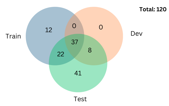
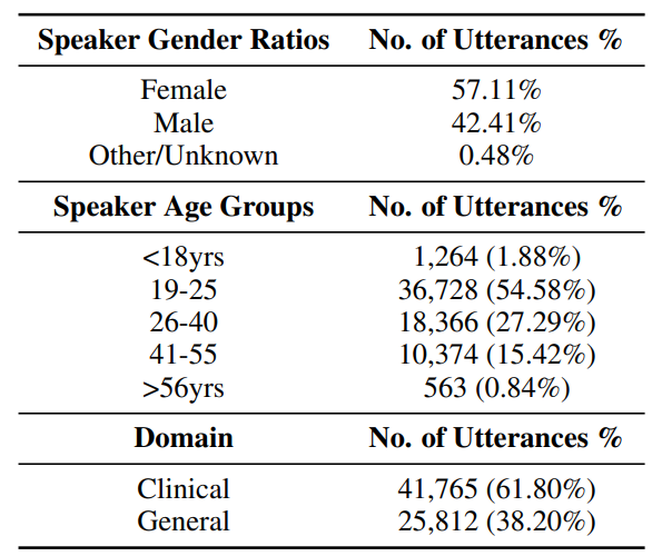
We use the Afrispeech-200 dataset (Olatunji et al., 2023b) for this work, an accented Pan-African speech corpus with over 200 hours of audio recording, 120 accents, 2463 unique speakers, 57% female, from 13 countries for clinical and general domain ASR. To the best of our knowledge, it is the most diverse collection of African accents and is thus the focus of our work. Table 1 shows the statistics of the full dataset and Table 3 focuses on the accentual statistics of the Afrispeech-200 dataset. With 120 accents, the dataset covers a wide range of African accents. The entire dataset can be split, in terms of accents, into 71 accents in the train set, 45 accents in the dev set and 108 accents in the test set, of which 41 accents are only present in the test set (see Figure 1). The presence of unique accents in the test split enables us to model them as Out Of Distribution (OOD) accents: a situation beneficial for evaluating how well our work generalizes to unseen accents.


3.2 Creating AccentFold
Obtaining and visualizing accent embeddings: AccentFold is made up of learned accent embeddings. To create the embeddings, we follow the work of Anonymous (2023). This is a multitask learning model (MTL) on top of a pre-trained XLSR model (Conneau et al., 2020). The MTL model contains a shared encoder with three heads : (1) ASR head (2) Accent classification head, and (3) Domain classification head. The accent classification head predicts over 71 accents while the Domain classification head predicts (binary) if a sample is from the clinical or general domain. The ASR head is trained with the Connectionist Temporal Classification (CTC) loss (Graves et al., 2006) using the same hyperparameters as Conneau et al. (2020). For the domain and accent heads, we perform mean pooling on the encoder output and pass this to the dense layers in each corresponding head. The accent classification head predicts over 71 accents with cross-entropy loss. Extreme class imbalance further makes the task challenging. Therefore, we add a dense layer to our accent classification head to model this complexity. Domain classification uses a single dense layer with binary cross-entropy loss. The 3 tasks are jointly optimized as follows:

We found the above relative weights to give us the best results. For all the experiments, we train the models with a batch size of 16 for 10 epochs. Following Conneau et al. (2020), we use Adam optimizer (Kingma and Ba, 2014) where the learning rate is warmed up for the first 10% of updates to a peak of 3e-4, and then linearly decayed over a total of 30,740 updates. We use Hugginface Transformers to implement this (Wolf et al., 2020).
We train this model on the AfriSpeech-200 corpus (Olatunji et al., 2023b). We then extract internal representations of the last Transformer layer in the shared encoder model and use these as our AccentFold embeddings. For all samples for a given accent, we run inference using the MTL model and obtain corresponding AccentFold embeddings. For a given set of accent embeddings, we create a centroid represented by its element-wise medians. We select the median over the mean because of its robustness to outliers.
To visualize these embeddings we use tdistributed stochastic neighbor embedding (t-SNE) (van der Maaten and Hinton, 2008) with a perplexity of 30 and early aggregation of 12 to transform the embeddings to 2 dimensions. Initially, we apply the t-SNE transformation to the entire Afrispeech dataset and create plots based on the resulting twodimensional embeddings. This step enables us to visualize the overall structure and patterns present in the dataset. Subsequently, we repeat the transformation and plotting process specifically for the test split of the dataset. This evaluation allows us to determine if the quality of the t-SNE fitting and transformation extends to samples with unseen accents.
This paper is available on arxiv under CC BY-SA 4.0 DEED license.

